Difference between revisions of "Flow Charts"
Jump to navigation
Jump to search
(Added some details) |
(new example) |
||
| Line 1: | Line 1: | ||
< [[MetaFun]], [[Graphics]] | < [[MetaFun]], [[Graphics]] | ||
| − | Context provides a charts module to create flow charts. For example | + | Context provides a charts module to create flow charts. |
| + | The details are in the [http://www.pragma-ade.com/general/manuals/mchart.pdf Charts uncovered] manual by Pragma. | ||
| + | There is also [http://www.im.ps.pl/context/?en Flowchart creater] to create flowchart code using javascript. | ||
| + | |||
| + | For example | ||
<context source="yes"> | <context source="yes"> | ||
| Line 24: | Line 28: | ||
</context> | </context> | ||
| − | The | + | The more sophisticated example: |
| + | |||
| + | <context source="yes"> | ||
| + | \usemodule[chart] | ||
| + | |||
| + | \setupFLOWcharts | ||
| + | [nx=5, | ||
| + | ny=3, | ||
| + | dx=2\bodyfontsize, | ||
| + | dy=2\bodyfontsize, | ||
| + | maxwidth=\textwidth | ||
| + | ] | ||
| + | |||
| + | \setupFLOWshapes | ||
| + | [framecolor=black, | ||
| + | background=color, | ||
| + | backgroundcolor=white, | ||
| + | ] | ||
| + | |||
| + | \startFLOWchart[DSP] | ||
| + | |||
| + | \startFLOWcell | ||
| + | \name{input} | ||
| + | \location{1,1} | ||
| + | \shape{44} | ||
| + | \connection[rl] {lowpass1} | ||
| + | \comment[t]{$x(t)$} | ||
| + | \comment[b]{$X(t)$} | ||
| + | \stopFLOWcell | ||
| + | |||
| + | \startFLOWcell | ||
| + | \name {lowpass1} | ||
| + | \location {2,1} | ||
| + | \text {Low Pass\crlf Filter} | ||
| + | \connection[bt] {adconv} | ||
| + | \comment[r]{$x_f(t)$} | ||
| + | \comment[l]{$X_f(t)$} | ||
| + | \stopFLOWcell | ||
| + | |||
| + | \startFLOWcell | ||
| + | \name{adconv} | ||
| + | \location{2,2} | ||
| + | \text{Analog/Digital\crlf conversion} | ||
| + | \connection[rl]{dsp} | ||
| + | \comment[t]{$x[n]$} | ||
| + | \comment[b]{$X(\Omega)$} | ||
| + | \stopFLOWcell | ||
| + | |||
| + | \startFLOWcell | ||
| + | \name{dsp} | ||
| + | \location{3,2} | ||
| + | \text{Digital Signal\crlf Processing} | ||
| + | \connection[rl]{daconv} | ||
| + | \comment[t]{$y[n]$} | ||
| + | \comment[b]{$Y(\Omega)$} | ||
| + | \stopFLOWcell | ||
| + | |||
| + | \startFLOWcell | ||
| + | \name{daconv} | ||
| + | \location{4,2} | ||
| + | \text{Digital/Analog\crlf Conversion} | ||
| + | \connection[bt]{lowpass2} | ||
| + | \comment[r]{$y_d(t)$} | ||
| + | \comment[l]{$Y_d(t)$} | ||
| + | \stopFLOWcell | ||
| + | |||
| + | \startFLOWcell | ||
| + | \name {lowpass2} | ||
| + | \location {4,3} | ||
| + | \text {Low Pass\crlf Filter} | ||
| + | \connection[rl]{output} | ||
| + | \comment[t]{$y_f(t)$} | ||
| + | \comment[b]{$Y_f(t)$} | ||
| + | \stopFLOWcell | ||
| + | |||
| + | \startFLOWcell | ||
| + | \name {output} | ||
| + | \location {5,3} | ||
| + | \shape{44} | ||
| + | \stopFLOWcell | ||
| + | |||
| + | \stopFLOWchart | ||
| + | |||
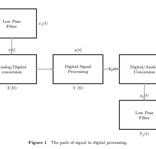
| + | \placefigure[here][fig:chart]{The path of signal in digital processing.} | ||
| + | { | ||
| + | \FLOWchart[DSP] | ||
| + | } | ||
| + | </context> | ||
| − | |||
[[Category:Graphics]] | [[Category:Graphics]] | ||
[[Category:Metapost]] | [[Category:Metapost]] | ||
Revision as of 17:00, 20 March 2008
Context provides a charts module to create flow charts. The details are in the Charts uncovered manual by Pragma. There is also Flowchart creater to create flowchart code using javascript.
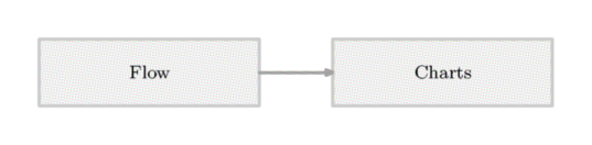
For example
\usemodule[chart]
\setupFLOWcharts[height=3\lineheight]

\startFLOWchart[example]
\startFLOWcell
  \name {flow}
  \location {1,1}
  \text {Flow}
  \connection [rl] {chart}
\stopFLOWcell
\startFLOWcell
  \name {chart}
  \location{2,1}
  \text {Charts}
\stopFLOWcell
\stopFLOWchart
\FLOWchart[example]
The more sophisticated example:
\usemodule[chart]

\setupFLOWcharts
[nx=5,
ny=3,
dx=2\bodyfontsize,
dy=2\bodyfontsize,
maxwidth=\textwidth
]

\setupFLOWshapes
[framecolor=black,
background=color,
backgroundcolor=white,
]

\startFLOWchart[DSP]

	\startFLOWcell
	\name{input}
	\location{1,1}
	\shape{44}
	\connection[rl] {lowpass1}
	\comment[t]{$x(t)$}
	\comment[b]{$X(t)$}
	\stopFLOWcell

	\startFLOWcell
	\name {lowpass1}
	\location {2,1}
	\text {Low Pass\crlf Filter}
	\connection[bt] {adconv}
	\comment[r]{$x_f(t)$}
	\comment[l]{$X_f(t)$}
	\stopFLOWcell

	\startFLOWcell
	\name{adconv}
	\location{2,2}
	\text{Analog/Digital\crlf conversion}
	\connection[rl]{dsp}
	\comment[t]{$x[n]$}
	\comment[b]{$X(\Omega)$}
	\stopFLOWcell

	\startFLOWcell
	\name{dsp}
	\location{3,2}
	\text{Digital Signal\crlf Processing}
	\connection[rl]{daconv}
	\comment[t]{$y[n]$}
	\comment[b]{$Y(\Omega)$}
	\stopFLOWcell

	\startFLOWcell
	\name{daconv}
	\location{4,2}
	\text{Digital/Analog\crlf Conversion}
	\connection[bt]{lowpass2}
	\comment[r]{$y_d(t)$}
	\comment[l]{$Y_d(t)$}
	\stopFLOWcell

	\startFLOWcell
	\name {lowpass2}
	\location {4,3}
	\text {Low Pass\crlf Filter}
	\connection[rl]{output}
	\comment[t]{$y_f(t)$}
	\comment[b]{$Y_f(t)$}
	\stopFLOWcell

	\startFLOWcell
	\name {output}
	\location {5,3}
	\shape{44}
	\stopFLOWcell

\stopFLOWchart

\placefigure[here][fig:chart]{The path of signal in digital processing.}
{
	\FLOWchart[DSP]
}